The Atmospheric Physics Behind Net Zero

The Atmospheric Physics Behind Net Zero

Professor Myles Allen

22nd November 2022

Welcome to the second Gresham lecture on net zero. I'm Myles Allen, the Frank Jackson Professor of the Environment at Gresham College, and I'm also a professor at the University of Oxford, and today I'm talking to you about the atmospheric physics behind net zero.

At the beginning of the last lecture, I talked to you about the different ways in which science progresses: by chance, by design, or by changing the subject. In this lecture, I'm going to talk a little bit about how occasionally science gets stuck, for interesting reasons. There are a couple of instances of how we've got stuck in the pre-history of net zero, which I'll be talking about today.

This history goes all the way back to the time of Joseph Fourier, of Fourier transform fame, Eunice Foote, and John Tyndall. These thinkers, in the early- to mid-19th century, were fascinated by the recently-discovered phenomenon of “invisible light”, infrared light that they couldn't see but which behaved in the same way as visible light.

Joseph Fourier speculated, without, as far as I can tell, any particular evidence, that certain gases in the atmosphere were responsible for absorbing infrared light and keeping the Earth warm, and hence is credited with having come up with the original idea of the greenhouse effect. A couple of decades later, an American scientist called Eunice Foote presented a paper called “Circumstances affecting the heat of the sun's rays”, which was the first empirical demonstration of the fact that different gases have a different impact on temperature, and that carbon dioxide was particularly effective at keeping things warm. Interestingly, I don't have a picture of her.[1] And also, for reasons that aren’t entirely clear, she never got to read her paper to the American Association for the Advancement of Science: Professor Joseph Hendry read it for her.

Fortunately, as far has women in science are concerned, things have moved on (at least a bit), but we can also bicker about whether Foote really demonstrated the greenhouse effect. She definitely demonstrated that carbon dioxide and water vapor had a different impact compared to, say, dry air, on the temperature of a thermometer exposed to the heat of the sun's rays. But just a few years later (and because there was no internet back then, he can't have known of Foote's experiments) an Irishman called John Tyndall was, in my view at least, the first to really demonstrate how different gases affect infrared light.

Tyndall did a number of elegant experiments and left us some beautiful drawings, including this one: if you look on the right here, there's a block of metal which is being heated by a gas flame underneath it. The infrared light from that hot body is going through that long pipe and being measured by that thermopile, the two cones at the other end. Tyndall is passing gases through the pipe to see what they did to the passage of the infrared light. And what he was able to show, with this very ingenious experiment, was that even if you could see through all these gases perfectly well with your eyes, for infrared light, it made a huge difference what gases he put into the pipe. In particular, he showed that carbon dioxide was a very effective blocker of infrared light.

Tyndall’s experiments were taken up by another 19th century scientist, this time a Swede, Svante Arrhenius, who gave the first quantitative account of the impact of increasing carbon dioxide on global temperatures. To quote from his paper: "Any doubling of the percentage of carbon dioxide in the air would raise the earth's temperature by four degrees, and if the carbon dioxide were increased fourfold, it would increase temperature by eight degrees." It almost reads like a sentence out of a modern climate science paper.

This was 1898, so it's extraordinary how long ago we've understood this. Interestingly, Arrhenius thought that doubling carbon dioxide concentrations would take 1,000 years or so, because of course he couldn't possibly anticipate that coal, oil, and gas use would explode in the late 20th century. Also, being a Swede, he thought a bit of global warming would be a good thing. Attitudes have changed.

But what's really interesting from the point of view of how science develops is that unfortunately Arrhenius didn't really get to bask in the glory of his discovery for very long, because an even more famous Swede intervened: Ångstrom, someone who'd be very well known to any chemist. Ångstrom was skeptical of Arrhenius's ideas, so he repeated Tyndall's experiment having worked out that between him and space was about two meters of carbon dioxide. What I mean by this is that, if you took all the carbon dioxide in the atmosphere and brought it down to the surface, so you had a pure carbon dioxide layer and no carbon dioxide above it, that layer would have been about two meters thick back then. It's about three meters now.

Because they understood the absorption of infrared light in gases quite well by this stage, Ångstrom also understood that it didn't really matter how long the path was. What mattered with the amount of coloured stuff in the way (thinking of infrared light as just light of a different colour). If that sounds implausible to you, imagine peeing in a white bucket full of water. The colour looking down into the bucket doesn't depend on the amount of water in the bucket to start with, it depends only on the colour and quantity of your pee. Feel free to try this at home if you don't believe me.

Ångstrom had the idea of, in effect, bringing all carbon dioxide in the atmosphere down to the surface, and then checking to see how much infrared light it was actually absorbing. And what he found was that absorption was almost complete: almost none of the infrared line got through. And if he doubled the amount of carbon dioxide, still none of it got through. And if he added water vapor, even less of it got through.

So Ångstrom published a paper saying, "Well, Arrhenius had an interesting idea, but actually all of the infrared light gets absorbed by the combination of carbon dioxide and water vapour, so adding more carbon dioxide can't possibly make any difference, so the carbon dioxide theory is rubbish." Which sounds very plausible. In fact, so plausible that for 50 years people largely forgot about Arrhenius's theory. So poor old Arrhenius went to his grave with no idea that he'd actually discovered something important.

Speaking personally, this is important to me because every now and then a physicist somewhere in the world rediscovers Ångstrom's argument and writes me an angry email saying, "Climate scientists are all incompetent. You obviously haven't thought about band saturation, and so global warming cannot possibly be caused by rising carbon dioxide." And it's understandable that people have this confusion, because the standard schoolbook picture we have of how the greenhouse effect works (apologies to “Encyclopaedia Britannica”) does indeed imply that the overall infrared opacity of the atmosphere, meaning the amount of infrared light that gets through the atmosphere from the surface to space, that somehow determines the Earth's surface temperature.

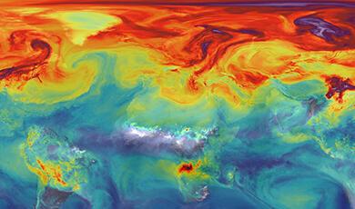
If we look at the planet in the infrared from space, you can see the daily cycle of cloudiness: those white blobs correspond to cold high clouds. You can see the swirls of weather motions in the atmosphere and so on. But what you can't see is the surface. So Ångstrom was right. The atmosphere is, for all practical purposes, almost opaque in the infrared.

At this point, when I'm giving this lecture to students, some of them start shifting in their seats and wondering if I'm sponsored by a major oil corporation. But before you switch off and decide that global warming's not a thing after all, I'm now going to tell you how it actually does work. It's not that much more complicated than the schoolbook picture.

Carbon dioxide is well mixed through the atmosphere, meaning the proportion of air that is carbon dioxide is the same whatever altitude you're at. So, if I just take a square column of atmosphere, and I represent carbon dioxide molecules by these coloured balls, it looks like this. The temperature of the molecules is indicated by the colour of the balls, and the absorption density (which you can think of as analogous to the density of pee in the bucket: it varies in the vertical a bit faster than the actual density, but that’s a detail) is indicated by the density of the coloured balls.

Before I go any further, the depth of the atmosphere is many kilometres, so these coloured balls, as shown, are hundreds of meters across. I originally made this graphic to give a presentation to a San Francisco court because I was tasked with explaining how the greenhouse effect works. Afterwards, Rush Limbaugh, a very strong-willed radio host in America, got very angry about the fact that I was a typical climate scientist exaggerating the problem of global warming by making out that carbon dioxide molecules are much bigger than they really are. So, I should warn you, these molecules are not to scale.

Temperature and absorption density of carbon dioxide molecules both decrease with height. If we look from the side, you can see that progression as you go up through the atmosphere. It gets colder with height. You've all experienced that if you've climbed a mountain: roughly six degrees Celcius per kilometre. And the density falls off as well, not at a constant rate like temperature, but exponentially, meaning a rate that depends on the density itself, because air is sitting under its own weight.

Now, imagine what's going to happen if you look down at this “ball pit” from above. Here's the actual view. You see a bunch of colours. What you don't see are those bright reds at the surface. You can't see through the atmosphere (on this point, Ångstrom was right). What you see, if you fuzz your eyes a bit, is the average colour of the balls that are visible from space.

If we flip that around, each of these colours represents a temperature. The balls (or molecules) all releasing energy. The hot (red) ones are releasing energy faster than the cold (blue) ones. The average rate at which the Earth is sending energy back out into space is determined by the average temperature of the molecules (or the average colour of the balls) that are “visible” (in the infrared) from space.

So far so good. The rate of energy emitted to space depends on the average temperature of the molecules that you can see from above. So, as we increase the concentration of carbon dioxide, what happens? If I double the density of carbon dioxide molecules everywhere, I can't see as deep into my ball pit. What that does is it forces energy to escape from a higher altitude. The carbon dioxide molecules you can see from space are colder, so they're not releasing as much energy.

Higher air is colder, and so it's radiating less energy back out into space. So, as we double carbon dioxide concentrations, we reduce the amount of energy going back out into space: same energy in, less energy out: global warming. This story has not mentioned the amount of infrared light going all the way through the atmosphere in either direction.

So, Ångstrom was wrong (you can tell me at the end why his experiment was misleading, that's a little challenge to you to think about through the rest of the lecture). Increasing carbon dioxide concentrations creates an imbalance. Same energy coming in, less energy going out. The system has to warm up, because energy is accumulating in the climate system. How much it warms up, we'll come on to. But it has to warm up a bit. And here is the atmosphere warming up to restore the balance, to make those balls the same average colour when viewed from space, as they were before carbon dioxide concentrations increased.

You are seeing different balls, at different altitudes. You're not seeing as deep into the atmosphere, but because we’ve warmed it all up, you're seeing, on average, the same colour of balls, the same temperature of molecules, as you saw before. And even better, from the point of view of explaining Arrhenius's theory, if you double it again, you actually get the same reduction in temperature, or change of colour, when viewed from space.

So, we've explained two aspects of Arrhenius’ theory. One was that increasing carbon dioxide would increase global temperature. The second is that every doubling of carbon dioxide concentrations, even though it would take twice as much extra carbon dioxide in the atmosphere to achieve, would have about the same impact on the global energy budget as the last one.

If this has all seemed a bit bemusing, don't panic. This is very well-understood science. I just wanted to stress it here because I think it's quite an interesting story about how a very eminent scientist, Ångstrom was a Nobel Prize winner no less, parked the whole carbon dioxide theory for 50 years with an elegant experiment that just missed out one crucial detail, which is the interplay between temperature and density through the atmosphere.

Even if you found this a little bit confusing, you don't need to worry about it because we've actually seen the impact of rising greenhouse gases from space. This is a remarkable observation, mostly because of the ingenuity of the scientists and engineers in the late 1960s. They flew an infrared interferometer, a delicate, complicated instrument that you would normally require a lab to operate, on a spacecraft in 1970, an extraordinary achievement, and produced a spectrum of infrared light. That's a measure of how much infrared light was emerging depending on the colour, or the wavelengths, of that light.

27 years later, it so happens that the Japanese space agency flew a similar instrument. They didn't do it deliberately, but John Harries and Helen Brindley at Imperial College noticed that the same observation had been made separated by 27 years, so around 30 to 40 parts per million of carbon dioxide, not to mention changing concentrations of methane, CFCs, and so on. So the Imperial team were able to compare these two spectra, correct for the fact that the temperature was a bit different in the two periods, and see the reduction in outgoing energy that resulted from those extra greenhouse gases in the atmosphere.

So Arrenhius’ idea is not “just a theory”: we can see it in action. We can see the impact of extra greenhouse gases on outgoing energy from our planet in precisely the wavelengths, or colours, of infrared light that we expect to see that reduction. So, we're completely confident in this part of the story: as we increase carbon dioxide concentrations, we slow down the rate at which energy escapes to space, creating an imbalance between incoming energy from the sun and outgoing energy to space and thereby driving some global warming. I emphasize some because this explanation alone doesn't tell you how much global warming. To understand the response, we need a climate model.

 “Yale Environment 360” is a great website, but this headline “Can we trust climate models?”, annoyed me. Absolute trust is something you give to your priest or your partner. You don't trust a climate model. Perhaps Michael Lemonick meant “trust” in the sense of “can I trust this wooden bridge?” But then the answer would have to been analogous to “that depends on whether you want to walk or drive a tank over it”: models may be trustworthy for some purposes, but certainly not all.

“Trust” the wrong phrase to apply to a climate model. A model is a set of equations. It may require a computer to solve them, but that's all it is. And it doesn't always even need a computer to solve. What a climate model does is tell you how you should expect a representation of the climate system to respond when it is disturbed in various ways, such as by increasing carbon dioxide levels. We can represent the climate system using equations solved on a computer, or we can represent it, much more intuitively, using fluids and pipes.

In-lecture demonstration: I'm now going to introduce you to the Gresham Climate Model, which we'll be seeing much more of during these lectures. This represents a way of solving equations without using a computer. I’m using a computer to drive it, but the calculations themselves are being “performed” by the flow of the fluid in the pipes, because I imagine you have a better intuition of how fluid flows through pipes than you have about how energy flows through the global atmosphere.

This is a simulation of our global climate system. The red stuff, which you can see dripping in, represents energy. This is the energy flowing in from the sun, warming our planet. And down the bottom here, this is energy flowing back out into space. Can I ask you to ignore the cylinder over on the right-hand side. It's got a cork in it, so it's not doing anything.

We have a balance between energy coming in from the sun and energy flowing out into space, and this balance sets the planetary temperature, which is represented by the level of fluid in this pipe. If we crank up the power of the sun and we had the same processes controlling energy going back out into space, you can imagine the Earth is going to have to get warmer.

I'm now going to make one slight modification of this model in order to be able to do experiments with it, which is that this natural flow, which I'm showing you here, is about 240 watts per square meter of the Earth's surface. That’s two old-fashioned incandescent light bulbs beating down all the time, flowing in and flowing out.

The greenhouse effect today due to past emissions is about 2.5 to 3 watts per square meters, so 1% or so of that natural flow. To make this model “realistic”, I'd need a fire hose pumping fluid in, to represent the full natural flow. But most of that natural flow doesn't change. We're only going to focus on the things that do change. So, I'm going to replace this label and say, instead of the total energy coming in from the sun, this model will focus on the net extra energy flow in. That net flow could be altered by two kinds of changes.

A small increase in the power output of the sun, for example, that would increase the net energy flow in. But because it's the net energy flow in, it could also be increased by more greenhouse gases, reducing the energy flow out. Less energy flowing out or more energy flowing in: the impact on the net energy flow in is the same.

I’m also going to replace this label and say this represents the net energy flow back out into space due to increased global temperatures. Apart from this initial trickle, these additional flows represent extra energy flowing in and out, departing from equilibrium. And the level of fluid in the pipe, instead of representing the total planetary temperature, which is about 300 degrees (in “proper” temperature units of Kelvin), represents changes from that pre-industrial equilibrium state, in Celcius.

To avoid having to come equipped with a fire hose, we're showing you just small changes about the background states. I call them small in the context of total planetary energy flows, but 1% of the total energy through-put from the sun to space is still substantial in terms of impact on humanity.

Now, having set up what it all means, what happens if we increase the speed of the pump? Intuitively, you know what's going to happen, but I'm going to do it for you anyway. I've increased the speed of the pump. Is it doing what you expected it to do? Notice that the level of fluid in the pipe started to rise immediately, and then gradually stopped rising because the extra flow in at the top is being balanced by the extra flow being driven out by the extra pressure due to the additional depth. That corresponds to warmer temperatures in the planet forcing energy back out into space faster than they did before.

If I double carbon dioxide concentrations again, I increase the net energy flow in by roughly the same amount (that was Arrhenius very foresighted intuition). Notice we get about the same amount of warming for every unit increase in the energy flow.

Just as a warning, in case you're disappointed when you try this at home, if I was to use water for this demo, you wouldn’t see that simple relationship between fluid flow and the level of fluid in the pipe. Which reminds me, I should've prefaced all this (and apologies for forgetting) by saying this brilliant contraption was built by Benedict Pery of Oxford Physics and Toby Rowles of Durham Physics, and they had to think very hard about designing it to make sure it actually did solve the equations we wanted it to solve. In fact, when I first came up with the idea, I thought we’d just use water. But water immediately goes turbulent, and turbulence makes life difficult (that's a general rule of fluid mechanics). The fluid we're using here is a little bit viscous, which stops it getting difficult, so if you want to try this at home, use olive oil or something like that.

Anyway, we've captured the idea that as you increase the net energy into the climate system by increasing greenhouse gases, you require the Earth's surface temperature to increase in order to drive that energy out again to restore the balance between incoming and outgoing energy. So far so good. But with this system, we were able to do a little test: we raised the pump rate (greenhouse gas concentrations) a little bit, saw how the fluid level (global temperature) responded, and then we were able to predict how much the fluid level would increase if we raised the pump rate further.

Let’s restore the pump rate to its initial value, which corresponds to reducing greenhouse gas concentrations back to pre-industrial levels. When scientists were first thinking about the climate problem, back in the 1960s and 1970s, they were more in this situation. They could see global temperatures were fluctuating, just as we can see the level of fluid in the pipe is wobbling up and down. They understood how the system worked well enough to predict that rising carbon dioxide concentrations would cause some warming. But humanity hadn't actually dialled up the pump rate (increased net energy imbalance due to atmospheric pollution) enough to have had a significant impact on global temperatures by that time.

We understand fluid flowing in pipes pretty well. If you knew the viscosity of the fluid, the diameter of the pipes and so on, you'd be able to predict what would happen (that was, indeed, what Ben and Toby had to do before they built it). But with the climate system, there are a lot more processes involved. So how could scientists in the 1970s predict how much global temperatures would go up as we increase greenhouse gas concentrations when then were in this situation before any significant warming had happened at all?

That comes back to the modelling so I'll go back to the PowerPoint now, and switch off the annoying noise. You'll see plenty more of Ben and Toby’s model as these lectures progress. And if you're wondering what this is and why has it has a cork in it, all will be revealed in the ocean's lecture in January.

You don't need to trust climate models. This is a model. It's a plastic tube. If I asked you “do you trust this plastic tube?” you’d think it was a rather strange question. Here is another model: an equation representing the behaviour of this plastic tube. A model of our model, if you like. F is the extra flow we're putting in, h is the increased water depth, k is the openness of the outlet pipe, as it were the “willingness” of the outlet pipe to let fluid through it, which depends on the viscosity (syrupiness) of the fluid and the dimensions of the outlet pipe. If we put these things together, and the expected behaviour is fairly obvious. The faster the flow, the bigger the F, the higher the h, the more the fluid level in the pipe will raise. So that's a model of fluid flow through plastic pipes.

Here is another a model, the Earth's climate system in equilibrium. Notice it's very similar. This is the point. This system of fluid in pipes is solving the same equations. Equations are not things that mathematicians dream up to annoy people at school. They're actually what nature uses to govern our universe. And this is the equation, or approximately the equation, that governs our climate system in equilibrium. F now is that net additional energy flowing into the climate system, which might be due to a dialling up of the power output of the sun or a dialling up of greenhouse gas levels throttling outgoing energy to space: both cause a net energy input into the climate system. Remember, less energy out has the same net impact as more energy in.

Big capital T always refers to global average temperature, not an absolute temperature but a change in temperature above pre-industrial, which people refer to as the level of global warming. And lambda here is the sensitivity parameter. It's like k, and it's something that it's quite hard to go out and measure. It's just what determines the relationship between the “forcing”, F, and T, the temperature.

Lambda is a very important quantity that people have talked about for years: it denotes the extra rate at which the planet sends energy back out into space per degree of warming. A large lambda means the planet is very efficient at getting rid of energy by warming up, while a small lambda means the opposite. Remember I said at the beginning of the lecture I was going to talk about scientific cul-de-sacs. My personal view is that the climate science community's focus on pinning down the value of lambda and hence the so-called equilibrium climate sensitivity was one such cul-de-sac. But when we started thinking about the climate problem, this is the way we thought about it. We knew that as you increase the flow of energy into the climate system, temperatures would have to respond. And we asked, "Well, how much warming would we need to restore the balance between incoming and outgoing energy?"

Specifically, people asked the question, “if we were to double carbon dioxide concentrations, how much warming would we need to restore the balance between incoming and outgoing energy?” That's what's called the equilibrium climate sensitivity. I’m defining it here using exactly the same equation. I've just added these little suffixes here to say this is the special case where we haven't just added any old extra flow of energy, but we've specifically doubled carbon dioxide.

Doubling carbon dioxide concentrations and then holding them constant at their new level is a standard experiment that we can do with a climate model. We can't actually do it with the real world. We are in the process of doing something rather like it, but crucially, we aren't in a position with the real world to do what we can do with a climate model, which is to double carbon dioxide and then leave it indefinitely to see what happens.

Lambda, the sensitivity parameter, depends on lots of very uncertain processes. It depends on water vapor in the atmosphere. It depends on clouds. It depends on melting of snow, how fast sea ice retreats, how the rate of temperature change through the atmosphere adjusts and so on. I could spend a whole lecture talking about what determines lambda, but all you really need to know is the various things that determine lambda are uncertain, so lambda itself is uncertain.

Back in 1979, Jules Charney chaired a panel of the US National Academy of Sciences that estimated a range for lambda and hence the equilibrium climate sensitivity. This is the quantity that Svante Arrhenius said was about four degrees, remember? The Charney panel looked at Arrhenius's reasoning, and more quantitative work done in the 1960s and 70s by the likes of Suki Manabe, and decided Arrhenius’ estimate was a bit over the top. At the time, they had was two numerical computer simulations of the Earth's climate response to a doubling of carbon dioxide.

It's important to recognize that back in 1979 global warming was a model-based prediction. The blue here shows monthly temperatures since 1850. This is the modern record, so I don't know exactly what the record was like when Jules Charney was looking at it, but the important point was, it wouldn't have been any clearer than this, because we're talking 40 years ago. So, Charney et al weren't observing a global warming at the time. In fact, if anything, temperatures had been pretty stable for the previous 20 or 30 years.

Incidentally, there is a myth that the scientific community was predicting a global ice age in the 1970s. We do know that every time the weather got cold in the 1970s a newspaper ran an article saying we're going to get a new ice age. But that's just because that's what newspapers like to do. It's hard to find actual scientific articles predicting a new ice age. But what was very clear to the scientific community was what was happening to carbon dioxide, and they predicted that a likely outcome of rising carbon dioxide concentrations would be a global warming.

How much warming was far from clear. I actually remember when I was a graduate student in the late 1980s, one of the first lectures I went to, an eminent professor in Oxford chatting about this temperature record. And I remember him saying, "It's interesting, isn't it, how they always predict the warming starts right after the end of the data" in a sceptical tone.

Obviously were no longer in that situation, but back then, the likes of Charney were in a position where, if they were going to make a prediction of global warming, it had to be model-based because they really didn't have any direct observations of global warming to help them. And they just had two models. The 1.5 to 4.5 degrees Celcius range they gave was based on the fact that, of the two models they had, one of them had a climate sensitivity of two, the other one had a climate sensitivity of four. They thought, "Well, it's a bit silly just to give the range, so we'll add half a degree on either end." Having talked to Carl Wunsch, who was on that panel, I believe that was more-or-less their reasoning.

So, can we do better? Well, fast-forward 25 years or so, the reductio ad absurdum of this whole enterprise of using climate models to pin down the climate sensitivity was an experiment we led from Oxford back in the mid 2000s called climateprediction.net. Some of you may have actually participated (thank you). We generated many different versions of a climate model and distributed them all over the world to ask people to run them for us and send us the results. There was one even being run at the South Pole. They all doubled carbon dioxide and sent us back the warming they got.

These are the first results we got from the experiment, and showing a distribution of simulated equilibrium climate sensitivity. Remember, 1.5 to 4.5 degrees Celcius was Jules Charney's range. Arrhenius's estimate was four degrees. So, lots of model-versions were supporting Jules Charney's range, but what is interesting is this tail of possible warmings going out to some ridiculously high numbers. This caused a certain amount of consternation at the time because it showed how difficult it would be to pin down the risk of high climate sensitivity or a high level of warming if we were to stabilize greenhouse gas concentrations at any particular level.

And the latest generation of models, shown over here on the right, aren't really helping either. They're not going up to 10 degrees, but they are up at six degrees or so, well above the upper end of the range that most people think is plausible. So, equilibrium climate sensitivity is uncertain. But lots of things are uncertain. The real problem with the equilibrium climate sensitivity is not that it's uncertain, but that the uncertainty itself is contestable. It's difficult to get everybody to agree on what the uncertainty in the equilibrium climate sensitivity actually is. And this brings us to a really interesting problem in probability theory, which now I'm going to try to explain.

There are not that many problems in maths that we can understand unless we're pro mathematicians, but this is one of them. Suppose you're driving a car with a dodgy speedometer. You know, of course, that distance equals speed times journey-time, and you know you have 40 miles to go. The speedometer says your speed is somewhere between 20 and 40 miles per hour. So, the journey will take between one and two hours. So far so good. You're meant to arrive in 1 1/2 hours. What are the chances that you're going to be late?

Who'd like to answer the question? Someone be brave. By the way, I'm willing to accept either of the obvious answers, and I've got both of them covered up. So go for it. You can't go wrong. Just to remind you, the journey will take between one and two hours, you're going to be late if you arrive after 1 1/2 hours. What are the chances you're going to be late? Somebody said 50%, great, thanks. Do I have any other offers?

37 1/2%, assuming it's a uniform distribution.

Okay, so someone's concentrating. If you assume all arrival times in the range are equally likely, then the answer is indeed 50%. If you assume all speeds in the range are equally likely, then the answer is 33%, which is close enough to 37 for me. So, which is correct? All you're told is that it's a rubbish speedometer. If it says 30, the speed could be anywhere between 20 and 40. If that's all you're told, which of these probabilities is correct?

It gets even more interesting if we talk about smaller probabilities. Suppose you'll get fired if you arrive in more than 1.9 hours, a really bad outcome. What are the odds you're going to get fired? If you assume all arrival times are equally likely, then the answer is 10%, because 1.9 is 90% of the way between one hour and two hours. Makes sense? But if you assume all speeds are equally likely (I won't force you to do this one) it's about 5%, 5.2%, to be exact. So, there is a factor of two difference in the probability you are going to get fired just based on what you assume “ignorance” means?

Now, let's think of another problem which may seem slightly more relevant to this lecture. Today's level of energy imbalance due to human activity is, depending on exactly when you measure it from, roughly 2.8 watts per square meter. Just rearranging those equations from before, I'll call it Fnow. That's the extra energy flowing into the climate system as a result of past increases in greenhouse gas concentrations and other forms of anthropogenic pollution in the atmosphere.

If we were to stop the atmosphere changing and hold it at today's composition forever, how much warming would we get? Well, that's going to depend on this equilibrium climate sensitivity. Suppose the equilibrium climate sensitivity is somewhere between 1.5 and 4.5 degrees, and suppose the extra energy flow from a doubling of carbon dioxide is 3.7 watts per square meter, what are the odds of any given equilibrium warming with today's concentrations of greenhouse gases alone?

I should emphasise these are illustrative examples, so you can do the maths in your head: these are not the actual canonical distributions people accept at the moment. But they serve to illustrate the point: if we assume all values of lambda, the sensitivity parameter, are equally likely, we get a 7% risk of temperatures going above three degrees. If we assume all values of the climate sensitivity, the warming due to doubling carbon dioxide, are equally likely, what are you expecting here? Is that going to be a higher number or a lower number? Did somebody say higher? Well done. The actual number is 18%: more than a factor of two difference in the estimated risk of a warming greater than three degrees Celcius arising solely from what you assume ignorance looks like.

This is the problem with this equilibrium climate sensitivity. It's not just that it's uncertain. We deal with uncertainty all the time. It's that the uncertainty in the climate sensitivity itself is contestable because the answer seems to depend on subjective decisions about how you set the problem up. It's even contested whether it's contestable. There are people out there who say, "No, it's not contestable. this was all solved by Edwin Jaynes in 1970." Except that Jaynes's solution has been contested by a paper published by Alon Drury in 2015. So, the argument continues.

Over on the left of this figure, 2.6 to 4.1 degrees Celcius is the canonical range of climate sensitivity in the most recent report of the Intergovernmental Panel on Climate Change. It came out of a big study which was initiated in a meeting in a castle in Bavaria. The Max Planck Foundation gathered together all the scientists who'd been thinking about climate sensitivity, we talked about the different lines of evidence, and then a team from the meeting went off to develop this paper, Sherwood et al., which was the outcome.

I wasn't involved in the paper, I guess because the last thing you want on an author team is somebody who just sits in the corner and says, "This is all pointless. I don't care", but this happens to be my view on the distribution of equilibrium climate sensitivity. I think it's a daft question. And inevitably, as recently as a couple of months ago, a new estimate using identical data has emerged, but just using different statistical methods and assumptions, which gives a very different range.

Why does this matter? Well, back in 1992, 13 years after the Charney report but at a time when the only experiments we could do with climate models was double carbon dioxide and see how much they warmed up, the Rio Convention was written. That contained this crucial line that the parties were aiming for “stabilization of greenhouse gas concentrations in the atmosphere at a level that would prevent dangerous anthropogenic interference in the climate system.” And so the scientific community immediately thought, "Well, we've clearly got to work out what that level is," which meant we had to work out the equilibrium climate sensitivity. Fortunately, it turns out that we can work out what it takes to avoid dangerous climate change without ever knowing the equilibrium climate sensitivity. This is the “change of the subject” that we will be explaining in the next three Gresham lectures.

But like the thing from the crypt, the equilibrium climate sensitivity keeps coming back to haunt us. This very-long-term equilibrium response only matters if we actually stabilize atmospheric concentrations of greenhouse gases and allow the climate to re-equilibrate, which, as we will explain in the next lecture, could take many, many centuries. The breakthrough in the late 2000s was the realization that we can actually stop the warming well before restoring climate equilibrium if we reduce anthropogenic emissions to net zero. Unfortunately, there's a catch. That assumption was we were talking about net zero anthropogenic emissions, assuming that carbon dioxide that was taken up by plants or oceans would just count as natural uptake, even if it was being taken up faster as a result of the fact there was more carbon dioxide in the atmosphere.

We'll come back to this in the carbon cycle lecture, but when we published those papers, we naively thought people would be grateful to nature for carbon that was being taken up by trees growing faster as a result of past emissions and just regard it as something natural that was happening. But, of course, those trees belong to somebody or they belong to a country, and now those countries want to take credit for that carbon uptake. And suddenly everybody wants to say that any carbon taken up by anything anywhere is a negative emission and sell it on the offset markets. And if we carry on burning fossil fuels and just buying offsets with these natural absorptions being counted as a negative emission, we're right back to where we started, because then net zero only means stabilizing concentrations in the atmosphere, and it's very hard to predict when temperatures would stop rising if we were to do that.

I mention this at the end because it's not often that a basic problem of probability theory, (it's a variant of Bertrand's paradox, by the way) actually has an impact on global climate policy. And it even has an impact when you decide whether or not to check that box next time you take an air flight. Checking that box funds all kinds of fine projects, so why not do it anyway, but just remember it's not actually compensating for your emissions.

So that's what we've tried to cover in this lecture: how rising carbon dioxide concentrations actually cause global warming (as opposed to the incorrect schoolbook picture) and why the equilibrium climate sensitivity is still so hotly contested. That was the paradigmatic view of climate science, the problems we faced in the 2000s and why we changed the subject to net zero. And then finally, I added this point about how even quite fundamental thorny issues in probability theory can actually have big global policy implications. Thank you.

© Professor Allen 2023

[1] Interestingly, Google claims to have a picture, but the images that show up are either of Mary Foote Henderson, Eunice’s daughter, or (strangely) Theresa Malkiel, the founder of International Women’s Day.