Login
Login
The Incredible Sine Wave and its Uses

Share

- Details
- Text
- Audio
- Downloads
- Extra Reading
The beautiful sine wave turns out to have a huge number of practical applications, from the motion of springs, to waves in the sea, to sound waves, light waves and more. It is curious that the function which defines the sine wave, sin(x), comes from comparing the lengths of sides in right-angled triangles – just about the least curvy things you could imagine. How does that concept result in the lovely curve of the sine wave?
Download Text

The Incredible Sine Wave and its Uses
Professor Sarah Hart
23 May 2022
We’ve all seen a sine wave, but we also all learnt in school that “sine is opposite over hypotenuse”. So somehow this very un-curvy thing, a ratio of sides of a right-angled triangle (which associates, to an angle greater than zero and less than a right angle, a number strictly between zero and one), is related to a wave that goes on forever and takes both positive and negative values. But how? I’m going to give you a brief history of “sine”, to get us from triangles to sine waves and their huge range of uses. Along the way we’ll encounter archery, banned books, and the workings of the human ear.
The Beginnings of Trigonometry
The Ancient Greeks had triangles, but they didn’t have sin, cos, and tan. In spite of this, we often see Hipparchus, the Ancient Greek mathematician and astronomer, called the Father of Trigonometry. The reason for this is that he used chord lengths (distances between points on the circumference of a circle) in his astronomical calculations. He was an important astronomer; he was the first to calculate the precession of equinoxes, and he used estimates of the parallax of the sun to evaluate the distance from the Earth to the Moon at between 59 and 67 Earth radii – not bad when the true figure is around 60 radii. I won’t go into detail about his exact calculations with chords as they were somewhat involved, but to give an example of how chords could be useful, one way to find the distance from the Earth to the Moon is to calculate the parallax of the Moon. For this, observers at two points as far away as possible find the position of the Moon in relation to distant stars (distant enough that they appear to be at the same point in the sky for both observers). This gives you two angles in an isosceles triangle. The height will give the distance to the Moon, and you can find it by trigonometry if you know the base. The base is a chord of a circle made by slicing through the Earth. So we can see from this example that chords matter. Hipparchus even drew up a table of chords, unfortunately now lost, to aid in astronomical calculations.
The next step in our story was in India a few centuries later. Again, they started out with chords. Originally the ratio measured was the length of the chord compared to the radius of the circle. Over time they realized that a more useful quantity was the half-chord – this cropped up more often in calculations. We can see why this might be in the case where the circle is (a slice through) the whole celestial sphere. The part we can see is the hemisphere above the horizon, which we can insert as a diameter. The height of a given star when it’s at a given angle in the sky is then the half chord length. Drawing in that diameter results in a right-angled triangle with angle θ between the diameter and the radius r of the circle, and the half chord length L opposite the angle. So sinθ=Lr , and that’s how it relates to the half-chord calculation. A table of chord lengths has to assume a specific circle radius, but a table of sine values only depends on the angle, and we can recover chord lengths easily by scaling – the sine value means we don’t have to fix on a specific circle radius at the outset.
We can visualize the set-up of a chord bisected by a radius as rather like a drawn bow, where the arc of the circle is the bow and the chord is the bowstring, which when pulled back gives the two radii from the centre to the top and bottom of the chord, while the arrow points along the radius. This is why the old Sanskrit word for sine, jīvā, means bowstring (and there’s our archery link). As the mathematical knowledge moved through the ancient world, so did the word. It was transliterated into Arabic as jība, which is meaningless in Arabic so was read as the more familiar word jayb, meaning cavity or pocket. This was then translated into Latin as sinus (the latin word for cavity), and sinus became our English sine. The final step, abbreviation from sine to just sin seems to have been done first by English mathematician William Oughtred in his 1632 book Circles of Proportion and the Horizontal Instrument.[1]
This idea of half chord lengths also tells us how to think about the sines of angles that don’t appear in right-angled triangles. In a unit circle (a circle of radius 1), we can imagine a radius at angle θ to the horizontal; the point where the radius meets the circumference is at height sinθ above the horizontal. This straightaway tells us that sin0=0 and sin90°=1 . Then the height starts decreasing until sin180°=0 , at which point we move below the horizontal, so the height is negative, with sin270°= -1 , and back round until we complete the full circle. And by the way, the horizontal distance from the centre would be given by cosθ.
I’ve used degrees here, but these are a rather earth-centric unit for angles, based on the ancient observation that there are (about) 360 days in a year. A more mathematically meaningful way to measure angles is to think of how far round the circumference travelling a given angle takes you – this unit is called the radian. In a unit circle the whole circumference is length 2π , so 360° equals 2π radians. If you do this then given a particular angle, the angle itself tells you how far round the circumference you have travelled, sine of the angle tells you your current height above the centre, and the cosine of the angle tells you your horizontal distance from the centre. We can now create our graph of sine, by having a radius travel around the circle and plotting, for each angle x , the height sinx above the horizontal of the end of the radius. We recover the familiar sine wave.
We’ve seen that the sine function is useful in astronomy, but that’s just the start.
Applications of Trigonometry
Right back to Hipparchus, mathematicians laboured to produce tables of, first chord values and later of the trigonometric functions we use today, for use in applications, of which there are many. Astronomy has always played a very important role in civilizations across the world, not least because of its importance in religious ceremonies. The picture shown in the lecture is a late 16th century depiction of astronomers at the Istanbul Observatory[2]. Navigation at sea also involved detailed calculations requiring trigonometry, for example a course calculation might involve a situation where you know two sides of a triangle (not usually right-angled) and the angle between them. Finding the required bearing means you need to know the remaining angles, and they can be found using a trigonometric identity called the cosine rule[3]. The ship on the slide is called the Peter Pomegranate[4]. It was built in 1510 for the navy of Henry VIII.
A final application is in surveying and map-making. To make accurate maps, you need to measure distances accurately. But this is difficult to do directly, given the existence of hard-to-traverse regions like mountains, rivers, and forests. Luckily, surveyors and mapmakers long ago hit on the brilliantly simple method of triangulation to determine distances very efficiently. It relies on the fact if you know one side of a triangle and any two angles, then the triangle is uniquely determined, and the remaining two side lengths can be determined using, guess what, our friend sine. To make your map, you find a place where the land is very flat, obstacle-free and easy to traverse, and you measure a base line b very accurately between two points. Your associate then travels to a third point a few miles off (but still visible), and you now measure two of the angles in the triangle you have created, using a theodolite (the third angle comes free because angles in a triangle sum to 180° ). The Sine Rule of trigonometry says that asinA=bsinB=csinC (with the notation as in the diagram shown). Since we know b , we can now find the remaining lengths a and c . Then you can move on and use these new known lengths as the bases of more triangles, gradually constructing a whole network of triangulation points across a large area.
These calculations are fine as long as our triangles stay very small compared to the radius of the Earth. But during the Great Trigonometrical Survey of India, which began in 1802 and was finally completed in 1871, the triangles were so big that the curvature of the Earth had to be taken into account. In such cases, fortunately, a modified sine rule still holds.
We are very lucky nowadays to be able to travel to completely unfamiliar places and rely, much of the time, on our phones to tell us where we are. This is achieved by means of the Global Positioning System (GPS). It relies on the same basic triangulation ideas as early map-makers used. There is a network of satellites in Earth's orbit that send out signals. Your phone picks up the signals, and by measuring the time it receives them compared to the time they were sent, it can determine exactly how far you are from each satellite. For each satellite, that puts you on a sphere of a given radius. The intersection of these spheres pinpoints your location. The intersection of two spheres is a circle. Adding a third sphere reduces the possibilities to two points. With four satellites the position is specified uniquely. Of course, it's still useful to be able to read a map for the inevitable moment when you lose signal or your phone battery dies!
Making a Trigonometric Table
All of these applications means that it is vital to be able to find the sines and cosines of angles very accurately. For that reason, trigonometric tables became very important. Some of the earliest tables in Europe were produced by a mathematician and astronomer called Regiomontanus (1436-76). He wrote De Triangulis Omnimodis, which was the first book solely dealing with triangles and trigonometry. In it he said “You who wish to study great and wonderful things, who wonder about the movement of the stars, must read these theorems about triangles”. He also produced an early book of trigonometric tables, probably intended for use in astrology, which was published posthumously in 1490. A few decades later came Georg Rheticus (1514-1574). His tables, published in 1551, are a hugely impressive calculating feat, representing a division of the circle into tiny fractions of seconds of arc, and values given to high levels of precision. He wasn’t using quite the standard trig functions that we use today, and surprisingly, the book was actually banned by the Catholic Church. It’s probably not because of anything particularly salacious (or should I say sinful), but because Rheticus’s other claim to fame is being the sole pupil of Copernicus – he played a vital role in getting Copernicus’s work published. Copernicus was, let’s say, not absolutely approved of at the time. Much more extensive versions of Rheticus’s tables were published later, and happily they weren’t banned.
So how on earth were these tables produced? There were various ingenious techniques, and they relied on formulae that were developed precisely because of the need to create tables of sines, cosines and other trigonometric functions. For example, if you know the sine and cosine of an angle x , there are formulae to find the sine and cosine of 12x . If you know the sine and cosine of angles a and b , there are formulae to find the sine and cosine of a+b and a-b . This allows you to make deductions from known triangles. For instance, you can use Pythagoras’s Theorem to find the height of an equilateral triangle of side 1 (it’s 32 ). Therefore sin(60°)=32 and cos(60°)=12. Meanwhile the diagonal of a regular pentagon of side 1 has been known since the time of Euclid: it’s the golden number ϕ=12(5+1) . You can then find the height (it’s 125+25 ), and that gives you the sine and cosine of 72° . Using the difference formulae we can then get sin(12°) , and then we can use half-angle formulae to get sin(6°) and sin(3°) , and so on.
These tables were very useful in their own right, but before we move on I want to tell you about a calculating technology that made use of them as tools in a completely different way. Logarithms were first used in 1614, but in the quarter-century leading up to that, there was another method found and used to multiply large numbers. It used trigonometry to convert multiplication into addition and subtraction, and was called prosthaphaeresis. You take two large numbers, say 123 and 456. You scale by a suitable power of ten, in this case dividing by 1000, so that they become numbers between 0 and 1. Then you use your trig tables to find numbers x and y so that cosx=0.123 and cosy=0.456, using as much precision as your tables allow. Now we use a formula for products of cosines: cosxcosy=12(cosx+y+cosx-y) . We find x+y and x-y , and check the tables to find the cosines of these. Then add them up, halve the answer, and you’ve found 0.123×0.456 (or as good an approximation as your tables allow). Scale back up, in this case multiplying by 1,000,000, and you get the answer to the original problem: 123×456=56,088 . Ingenious!
From sin(x) to sine wave
We’ve seen the sine wave as a curve defined between 0 and 2π . But there are many physical systems that involve repeating, periodic motion, that turn out to involve the sine function. Two examples are springs and pendulums, whose oscillating motions correspond to a repeating sine wave. The reason for this is that the sine function turns out to be the solution to equations modelling systems where there is a force acting towards an equilibrium position, and that force is proportional to the distance from that position. In a simple pendulum, there are two forces acting: gravity, and the tension in the swinging rod. That tension exactly balances out the component of gravity along the radius. The other component is acting along the circumference towards the lowest position of the bob: hanging vertically downwards. For small angles, to a good approximation, it is indeed proportional to the distance from that position. So we see a sine wave.[5]
The other example of springs has a Gresham connection, because it arises from Hooke’s Law. Robert Hooke was my predecessor as Gresham Professor of Geometry. He first published his law in 1676 in the form of a Latin anagram of the law – this sort of thing was quite common in those times because it was a way to establish priority. Hooke’s Law says “as the extension, so the force”: in other words, if you hang a weight from a spring, there will be an equilibrium point where the gravitational force downwards will exactly match the tension in the spring pulling upwards. If that equilibrium is disturbed, then the restorative force is proportional to the distance away from the equilibrium point. So, again, the position of the spring as it oscillates around the equilibrium point will relate to sin(t) where t is the elapsed time.
There are many other waves occurring in science and nature. Water waves are complicated and difficult to analyse, because there are lots of forces acting (including gravity and wind, and for small waves surface tension also comes into play), but if the amplitude of the waves is small compared to their length, we do see a roughly sinusoidal shape. As the amplitude increases, the peaks become sharper and the shape closer to a curve called a trochoid.[6] There are many situations where we have a periodic (repeating) phenomenon that is not a sine curve. But it turns out that sine curves still have a part to play, because of a wonderful piece of mathematics discovered by Joseph Fourier.
The Amazing Fourier Series
Joseph Fourier (1768 – 1830) comes into our story exactly 200 years ago, in 1822, when he published a book, Théorie analytique de la chaleur, on the mathematics of heat flow. There is an equation called the heat equation governing the way heat passes through solid bodies, and in trying to solve this Fourier was working with sine waves. There are ways you can modify the initial curve y=sinx . (And all this goes for the cosine function too, because cosx is just sin90-x , so the graphs are exactly the same, just shifted a little along the axis.) The graph y=2sinx, for example, is just the original curve doubled in height – we can think of a circle of twice the radius – while the graph y=sin(2x) represents travelling twice as fast around the circle. You can also add sine waves together (as long as their periods are the same or have a common multiple), and the result will be a periodic function, potentially more complicated but still periodic. What Fourier showed was the incredible fact that essentially any[7] periodic function can be expressed as a sum of sine waves. Even better, there is a straightforward process to find exactly which sine waves are required to obtain the so-called Fourier Series for the function. We showed in the lecture that you can make a square wave from adding the sine waves sinx+13sin3x+15sin5x+… . This is about as far from the sinuous sine curve as one can imagine for a periodic function. We also saw the sawtooth wave, which is obtained from the series sinx+12sin2x+13sin3x+… , which is almost the converse of our initial question of how do we get sine waves from right-angled triangles. Now we’ve managed to get right-angled triangles from sine waves!
Sound and Music
I want to finish up with looking in slightly more detail at a subject involving lots of sine waves: sound and music. It’s been known for a long time that there is a connection between musical pitch and frequency. Pythagoras did experiments with a simple stringed instrument called a monochord, where he found that changing the length of strings can affect the pitch in a specific way, and that certain simple ratios of lengths sound particularly pleasing together. We talked about maths and music at length in some of my previous lectures, so I won’t go into all the details now, but for example, if you halve the length of a string, the sound produced sounds very similar to the initial sound – we now know the frequency doubles, and the sounds we would say are an octave apart. Other pleasing ratios are 3:2 and 4:3. It was not clear why, though.
Many worked on the questions of frequency and harmony, including Galileo and Mersenne. One important name in the story is Joseph Saveur (1653-1716), who coined the term acoustics. He was fascinated by sound and did significant work in this area in spite of, or perhaps because of, his significant hearing impairment. He carried out detailed and very accurate experiments on frequencies, including what one account called “the nodes of undulating strings”. He noticed that depending on how you pluck the string initially, you can get places along the string where the string is almost still – he actually put little pieces of paper on the strings to test this. These places were always equally spaced along the string, so you might get the midpoint, or the points one-third and two-thirds of the way along the string, and so on. It was a mystery as to why this might be, until the French mathematician Jean-le-Rond D’Alembert (1717-1783) came along, and found a method to solve the equation governing motion of vibrating strings.
If you take a string fixed at both ends, like a violin string, and disturb it at time t=0 , then the vertical displacement y at a point x along the string depends in a very specific way on both x and t . The relationship is given by the so-called wave equation, and D’Alembert found a way to solve it. He showed that any solution to the equation is the sum of two waves moving in opposite directions along the string. When wave A gets to one end of the string, because the end cannot move, it must be precisely cancelled out by an inverted wave B travelling in the opposite direction. The whole thing happens again at the other end of the string, and wave B is reflected to produce wave A again. This means that the solution as a whole must be periodic with period 2l , where l is the length of the string.
Thanks to Fourier, we can then deduce that every solution is a sum of sine waves with period 2l (or more accurately a whole number of their periods must equal 2l ). So Saveur’s bits of paper were exactly showing the zeroes of the different possible sine waves. The different possibilities correspond to frequencies f , say, for the longest possible sine wave, and then 2f , 3f , and so on. Different instruments have different combinations of these waves – the fundamental frequency is the largest, and there are different proportions of the multiples, or harmonics. The fact that any note played has multiples of its fundamental frequency hidden within it means that a note whose basic frequency is 2f or 32f , for example, will share many of the same harmonics, and that’s one reason why these combinations sound pleasing together.
Synthesisers can use Fourier analysis to break down the sound made by different instruments into their component sine waves, and then reproduce those sounds by putting them back together.
We end with a brief discussion of how the ear processes sound. After Fourier discovered that any periodic function can be broken up into constituent sine waves, Georg Ohm (1787-1854) proposed that the ear itself breaks down notes into their component pure tones – this is known as Ohm’s acoustic law. Then Hermann von Helmholtz (1821-1894) built on this, giving a description of how the brain determines the frequencies of sine waves, which is known as the place theory of perception of pitch. To cut a long story very short, in the cochlea of the inner ear, shown in the diagram[8], there are two parts divided by the basilar membrane, which narrows at one end, and has tiny hairs on it. As sound enters the ear, it causes the fluid in the cochlea to vibrate and the basilar membrane to move up and down. As the membrane narrows, each individual frequency will reach a point where the space is too small for a wave of that frequency to be sustained. At that point the membrane must absorb this motion, which causes the hairs there to move more, triggering the nerve endings to send messages to the brain. From detecting which hairs are sending the signals, the brain experiences the different sounds. This theory was supported by experiments done in the 1950s by the Hungarian scientist Georg von Békésy (1899-1972), research which contributed to his being awarded a Nobel Prize. What all this means is that your ear is constantly doing Fourier analysis and decomposing sounds into sine waves. In fact, without sine waves, you wouldn’t have been able to listen to me talking about them today.
© Professor Sarah Hart, 2022
@sarahlovesmaths
References and Further Reading
Kim Plofker’s excellent book Mathematics in India (Princeton University Press, 2009) includes detail on trigonometry in Indian mathematics.
A good starting point for biographical information on historical mathematicians is the MacTutor History of Mathematics Archive. https://mathshistory.st-andrews.ac.uk/
David J. Benson, Music: a mathematical offering has a lot about acoustics and the applications of the sine curve in music.
Joseph Fourier’s 1822 Théorie Analytique de la Chaleur was reissued by Cambridge University Press in 2009, along with Alexander Freeman’s 1878 translation, The Analytical Theory of Heat. The original 1878 book is out of copyright so digitized copies are freely available online.
You can experiment with square and other waves using the Fourier Series Calculator at https://www.mathsisfun.com/calculus/fourier-series-graph.html.
My past Gresham lectures on music (and lots of other things!) are at the Gresham college website.
[1] Oughtred is also given credit for inventing the slide rule, in about 1622.
[2] Public domain image: https://commons.wikimedia.org/wiki/File:Taqi_al_din.jpg
[3] If sides a and b have angle θ between them, and the unknown side is c , then c=a2+b2-2abcosθ . Once all three sides are known the same rule can be redeployed to find the remaining angles.
[4] https://en.wikipedia.org/wiki/Peter_Pomegranate
[5] The spring animation in the lecture is by Svjo, CC BY-SA 3.0. The pendulum animation is by Wikinana38, CC BY-SA 4.0, both via Wikimedia Commons.
[6] For more on this, see http://hyperphysics.phy-astr.gsu.edu/hbase/Waves/watwav2.html
[7] For mathematicians watching – it’s not quite “any”. We can think of weird exceptions that don’t work, on purpose to be difficult. For example, we could define a periodic function f by letting f(x) = sinx when x is rational and f(x) = 0 when x is irrational. There are necessary conditions for a Fourier series to exist, called the Dirichlet conditions, which specify what is required – things like being continuous at all but a finite number of points. Any “naturally occurring” periodic function is going to be fine.
[8] The diagram is from the 1918 edition of Gray’s anatomy, which is in the public domain.
References and Further Reading
Kim Plofker’s excellent book Mathematics in India (Princeton University Press, 2009) includes detail on trigonometry in Indian mathematics.
A good starting point for biographical information on historical mathematicians is the MacTutor History of Mathematics Archive. https://mathshistory.st-andrews.ac.uk/
David J. Benson, Music: a mathematical offering has a lot about acoustics and the applications of the sine curve in music.
Joseph Fourier’s 1822 Théorie Analytique de la Chaleur was reissued by Cambridge University Press in 2009, along with Alexander Freeman’s 1878 translation, The Analytical Theory of Heat. The original 1878 book is out of copyright so digitized copies are freely available online.
You can experiment with square and other waves using the Fourier Series Calculator at https://www.mathsisfun.com/calculus/fourier-series-graph.html.
My past Gresham lectures on music (and lots of other things!) are at the Gresham college website.
Part of:
This event was on Mon, 23 May 2022

Support Gresham
Gresham College has offered an outstanding education to the public free of charge for over 400 years. Today, Gresham College plays an important role in fostering a love of learning and a greater understanding of ourselves and the world around us. Your donation will help to widen our reach and to broaden our audience, allowing more people to benefit from a high-quality education from some of the brightest minds.