Login
Login
Compression
Share

- Details
- Text
- Audio
- Downloads
- Extra Reading
When you tune into Netflix you might not be aware that the box in your living room starts a complex set of negotiations with servers on moving 563 Gbytes of information into your residence. That is equivalent to having 15,000 copies of the Encyclopaedia Britannica dumped into your home! So, why is watching a Netflix film not the equivalent of the Amazon-delivery from hell? Compression, which this lecture will show is economically and entropically a hot topic.
Download Text

It’s evening, you fancy watching a film[1], Netflix beckons, you kick off your shoes and tune-in to the latest 4K blockbuster. “Click!” – you press the button and, with no fuss at all, a modern digital miracle happens: terabytes of video, audio and text are shuffled around the planet, your internet connectivity is measured and in less than a second you are watching “Scream V” in 4k UHD video and 5.1 audio. It’s a modern marvel, because that blockbuster occupies terabytes of space on the Netflix video servers, yet you are connected by a piece of wet string and Wi-Fi. What makes this is all possible is compression – the unsung technical hero of the internet. Nothing works without compression and that was this lecture is about.
Let’s try and put some numbers on it. The latest Bond film “No Time to Die” has a running time of 163 minutes. Let’s assume we are watching it in 4K resolution. 4K video is 3840 by 2160 pixels = 8294400 pixels. Let’s assume 8 bits (although it could be more) per colour channel = 24 bits per pixel, and let’s take a frame rate of 50Hz. So that is 829440 ´ 24 ´ 50 roughly equals 10 Gbits s-1 which means the whole movie accounts for 100 Tbits. Of course, were we to measure the size of the original film, which was probably filmed at a considerably higher resolution and colour depth, then it is easy to find digital assets which exceed petabits (that’s 1015). Now, back to Netflix, you have pressed the button and you want 10 Gbits s-1 to arrive down your 25 Mbits s-1 cable. Somehow, we need to compress the video by a factor of 400 – a 400 to 1 compression ratio.
In the slides I demonstrate what 400:1 looks like. I randomly deleted pixels in the same ratio and the resulting image is incomprehensible. Yet the images we look at everyday are indistinguishable from the original. A further cleverness is that the encoder may not know precisely how your decoder will fill in the gaps – think of YouTube where you might be using any number of platforms and operating systems. How can the encoder remove information without the decoder having intimate knowledge of what it has done?
As is often the case with compression, well known compressors build upon other ones. So, to explain video coding, I first need to explain lossless coding. And, in order to explain that I need a simple domain - let’s pick text. In a previous lecture [1], I drew attention to the fact that written text contains characters at different frequencies. In French and English, “E” is the most common character[2]. In the most common encoding of text, which is called UTF-8, the uppercase and lowercase English letters are represented by an 8-bit word. On the face of this is a little strange, 8-bits are enough to represent 256 = 28 combinations and the letters a-z and A-Z is considerably less than 256 but even allowing for additional characters which are needed to represent returns, quotes, exclamation marks and so on, there is clearly some redundancy. Maybe we could use a much smaller number of bits for the letter “E” and for uncommon letters, such as “X” we could use more? Well, that’s an interesting idea but it leaves a few further questions? How can we create a unique code of variable length? Obviously, we cannot have a short code that is a prefix of any other code, or we will not be able to work out the joins between codes. And then there is the knotty problem of how to choose the length of the code in a way that is optimal?
Strangely the first person to examine this was an undergraduate called David Huffman at the Massachusetts Institute of Technology[3]. Huffman was able to show that his code reduced that amount of information and did so in a nearly optimal way [2]. Let’s take one of David Huffman’s original examples. For explanatory purposes let’s imagine we have only eight symbols in our alphabet which I’ll call ATCGSBZP. (Eight alphabet systems have recently come back to popularity via studies of DNA [3]). If we follow through the Huffman algorithm then we can see that, by using a variable number of bits per symbol, we save 0.2 bits per symbol — assuming our probability estimates are right. That might not sound very much but for a million symbols that is a saving of 200 kbits. And, on bandwidth sensitive applications such as broadcast radio, tv or satellite communications, that is definitely worth having. Eager readers are probably wondering if Huffman is the best compressor. And how would we know? Well, the polymath Claude Shannon looked at that question [4]. He made the following argument:
Let’s imagine we had a symbol appearing with a probability, p. Well, another way of writing that is p = 1/N where there are N possibilities. How many bits does it take to encode N possibilities? Well 2I, thus, with a smidgen of logarithms, we can show that I = -log2(p ). I is called the Shannon information, and it just another way of representing probability. If someone says something is one-in-a-million, you could equally well say it’s 20 bits. So, the average information for this code, which is sometimes called the entropy, is, according to my calculations, 2.75 bits. From which we know that there is around 0.5 bit per symbol missing.
To reach that lower limit, and not lose 0.5 bits per symbol, we need to switch to a coding system that is not restricted to modeling probabilities as powers of two — I did not prove this, but it is the case that Huffman is only optimal in the case that the symbol probabilities are exact powers of two. We’d also like to be able to realise some more gains by handling groups of symbols. And we’d like a system that, if the probability estimates are wrong, can adapt to the measured probabilities. All those features are found in arithmetic coding.
The concept behind arithmetic coding is represent a block of characters, or string as we call it in computer science, as a binary decimal number. A binary decimal number might something like .1101. By using a decimal, we can account for arbitrary probability distributions. The precise description of arithmetic codes is beautiful but very long (one of the more comprehensive YouTube tutorials takes at least five hours). Arithmetic coding represents the peak of achievement in general lossless coding and, if all we know are the symbol probabilities then arithmetic coding is a good choice.
Oftentimes however, we might know something more about the data. For example, if the data are human language, then we know that certain clusters of characters, words and sentences, are more likely than others. If we are dealing with speech, then we know there are periods of silence which do not require high-fidelity coding. Were we to consider a binary image, that’s an image with only black or white pixels, then we will have data with long intervals of repeats. We would say there are long runs of identical values. Hence run-length coding which codes every value with an additional number that is the length of the run. There are a few ways you can code it (some systems use Paris of numbers (value, run length), if there are only two values as in this example then you do not need to code the remaining values as one can flip the value at the end of each run). Run-Length Encoding or RLE used to be a popular coding method especially in the day of faxes and now survives via the TIFF pack bits option but in little else. This illustrates another useful point about compression – compression is often specific to the source and the technology – when technology changes the compression needs to change.
Another wheeze is to reorder the data before compression so that it is easier to compress. Maybe we could create runs, so that run-length coding might work better? On the face of it, this sounds tricky as we might end up sending as much data about the reordering as there are data itself! One particular piece of magic is the Burrows-Wheeler transform, as used in BZip (the B stands for Burrows Wheeler). It uses the data to re-order itself via a combination of cyclic shifts and permutations. For encoding the first stage is to put the data into blocks. We then create all the cyclic shifts of the block, sort them lexically and then the output is the final column of the data (which is the same size as the input data but with many repeated characters next to each other, which makes subsequent coding easier). Decoding is slightly more complicated – the data are put in a column and each row is sorted lexically, the data are then augmented by the input data again, which is added to the first column, and sorted. This is repeated until we have a block of data the same size as the input. The decoded sentence is the one that has the final symbol at the end of the sentence (Burrows Wheeler usually uses a special “end of block” marker so the decoder knows where to stop).
Lossless compression, with or without Burrows-Wheeler, is theoretically very attractive but it’s only really used in specialized circumstances when all the data must arrive intact. Examples might be when we are transferring files or when it is essential that all data arrives intact. A further issue with lossless compression is that the compressor must have an identical twin called a decompressor. This does not allow for much innovation – if a manufacturer designs a coder, then they had better build the decoder and the decoder had better exactly invert the coder. Lossy compression is quite different – the coder gives an impression of the signal, and the decoder reconstructs as best as they can.
In the modern world, by far the majority of compressors are lossy. The idea behind a lossy compressor is to model the imperfections of human perception. Just as a skilled illusionist can persuade the audience to fill in the gaps, a good lossy coder sends just enough information that the receiver believes the signal has been received. I hope it follows from that, that each signal domain has its own lossy compression – you would be unwise to use JPEG to compress a Beethoven symphony or CELP 32 to compress DNA sequences. One considerable downside of lossy compression for the educator is that the transmitted bitstreams can be very complicated. Because the coder and decoder are often made by different people, there are complex specifications for what must be sent, and the detail absorbs many a fun hour. My solution to this is to focus on only a few lossy compressors and steadfastly ignore the detail
The most famous of the lossy standards is JPEG which was named after the Joint Photographic Experts Group[4]. The group started its work in the mid-1980s and was led by Graham Hudson from British Telecom (in those days BT did research) [5]. There were several aspects of JPEG which have been widely copied subsequently but the first, and most obvious one if you have used it, is that it provides a “quality” parameter. As the quality is lowered, the size of the image decreases. In the lecture I show an image taken from an image compression test set [1]. Although it is not designed to win awards, the image is quite striking and shows a handsome lady striding off a ferry in Ho Chi Minh City dressed in some very natty pyjamas. Above her is the lowering tropical sky that is commonplace in Vietnam. The image was taken “raw” from a digital camera[5] and, by adjusting the JPEG quality threshold we can plot the reduction in size. The results are quite spectacular. Depending on the device on which you are viewing the slides, I would suspect that very few people would know, nor care, if the quality parameter was set as low as 30% which represents a compression ratio of 100:1.
If we zoom into the lady’s striped pyjamas then there are clues to how JPEG works – we can see a certain blockiness — but actually JPEG is a series of tricks that experience has found can fool the human eye[6]. In order of application these tricks are
- The eye does not have equal acuity in all colours. Although computers usually manipulate photographic images as three images, Red, Green and Blue (the RGB format), a better mapping to the human visual system is a luminance or brightness channel (usually denoted Y) and two other channels that contain only colour information. There are quite a few alternatives for those two channels, but the pair that JPEG chose, probably because of their legacy with old TV systems, are chrominance channels Cr and Cb (the red and blue chrominance). The eye is not as sensitive to spatial variations in chrominance, so JPEG allows coders to discard chrominance pixels if desired. This practice is quite commonplace in digital video processing, and you might see references to 4:2:2 4:2:0 video which, to the cognoscenti, reveal how much chrominance information has been discarded[7].
- JPEG dices the input image into blocks of 8 by 8 pixels[8]. JPEG then makes use an innovation that I will describe in a later lecture, an integral transform. It makes an assumption, which is that any eight-by-eight block can be exactly represented by a weighted summation of cosines. Fortunately, it turns out that we can compute the weights of those cosines very quickly indeed, and it is easily done in hardware, using the Discrete Cosine Transform or DCT. The DCT is a one-to-one transform meaning that the 64 input pixels generate 64 DCT coefficients — no saving there — but, very often, only a few DCT coefficients are needed to approximately represent a block which leads to potential efficiencies by not sending some coefficients or sending only approximations.
- Given a fixed number of bits, we can decide how to allocate those bits across the DCT coefficients. This is called quantisation. Because there are 64 numbers to be represented, we sometimes call these a vector – hence vector quantisation. Whole theses are written on interesting algorithms for vector quantisation and the JPEG standard doesn’t tell you how to do it, which means there is space for innovation and improvement. One simple method, which you can see from my examples in the lecture is to set small coefficients to zero.
- Generally speaking, the coefficients of the DCT that correspond to static or slowly varying components, will be much larger than the others. So, if we scan out the coefficients in the right way, we can cause there to be runs of similar coefficients which compress nicely.
- Use Huffman coding to compress the data.
Phew! What a complex sequence of steps. Notice that JPEG, like many successful coding standards builds upon other compressors – in this case Huffman coding which is used to squeeze any remaining redundant information out of the DCT coefficients. I have skipped a lot a detail here – I have not talked about the lossless JPEG modes, nor have I noted that JPEG does allow for arithmetic coding (although it is rarely used) not have I talked about JEPG2000 which is the successor to JPEG. However, the basic principle of block coding and the use of the DCT turned out to be critical and has been very widely copied in all commercial image and video coding standards.
I started this lecture with some observations about movies. The predominant coding standard for movies is MPEG (named after the Motion Picture Experts Group). MPEG has defined a series of coders from MPEG-1, now largely obsolete, MPEG-2 and MPEG-4. MPEG-4 was enacted as an ITU standard where is confusingly known as H264. It is also sometimes known as AVC or Advanced Video Coding. It has been estimated the over 90% of digital video in use today is transmitted using the H264 standard. The standard is multifaceted and has many parts and it is commonplace for manufacturers to claim that they have an MPEG-4 compliant coder when they are implementing only the easy bits![9] Nevertheless the principal idea, motion coding, is quite easy to illustrate.
As a movie is just a sequence of images, one of the simplest video coding standards merely uses JPEG to code each frame. Although though this, Motion-JPEG or M-JPEG, sounds a bit primitive, it is actually used, particularly in simple cameras such as those found in security systems. However, the real coding gains arise when we consider sequences of frames. I’ve taken one of the famous MPEG sequences[10], the “foreman” sequence to illustrate the problem. Although the camera is handheld (so moving a little), we can see that many of the eight-by-eight DCT blocks are little changed from frame to frame. Of those that have changed, they are well modelled by moving a block in one frame from somewhere else in a previous frame. That is what a good video coder does, it fully codes certain frames, MPEG calls them I-frames, and then it computes appropriate block movements from I-frames to construct the other predicted frames. If those predictions are good, then the coder does not need to send many corrections and bandwidth is saved. These movements are known as motion vectors and a fancy coder will conduct an expensive spatial search to find the best motion vectors. Note that the decoder need not be fancy – it just follows the instructions from the motion vectors. This is why encoding video on your computer is a slow process yet decoding can take place in real time on a computationally puny device such as your mobile phone.
In the MPEG parlance the frames that are estimated from the I frames are known as either P-frames, or B-frames. P-frames are predicted forwards from previous I-frames, whereas B-frames can be constructed from previous and future I-frames. This is potentially more efficient, but it implies a frame buffer to hold groups of incoming frames. This in turn introduces latency into the video chain which may be unacceptable in some circumstances[11]. What may not be obvious from the above description is that the amount of MPEG information transmitted depends heavily on the motion in the scene. If there is a jump-cut, then every block has to change and suddenly large amounts of bandwidth are required. For the internet this might not be so problematic, but for broadcast there may not be that much flexibility on bandwidth and blocks will be dropped. You may still see this on some live-event coverage – rapid camera pans, zooms, and jump cuts-can overwhelm the system and, at some vital sporting moment, our view is obscured with blocking artefact.
It goes without saying that evaluating lossy codecs is particularly challenging. Firstly, although there is an emerging science on what constitutes good quality, for the time being we rely on the judgements of humans. And measuring the performance of humans means entering the horribly equivocal world of psychology. Even if you step around that and use one of the proxies for visual quality such as PSNR, SSIM, or VMAF then you need to carefully control for rate, as some codecs work well for high-rate video and others well for low rate. Then there is computation. In broadcast, the compression must take place in realtime, so nebulous tasks such as “find the best motion vectors” have to constrained to “search in a such a way that you get a solution to all the vital motions vectors in a fixed time”. Thus, computational limits constrain visual quality. If the three-dimensional problem of quality versus rate versus computation is not challenging enough, then we should also mention that video compression results can vary dramatically by source material: compression algorithms that work for Formula 1 may not always work well for Antiques Roadshow.
A critical feature of lossy compression is that each type of source material demands a different compressor. This feature means regretfully I have to leave out discussion of audio compressors such as the ubiquitous MPEG Layer III (mp3). However, just as human speech audio sounds different to a symphony, there are specialist compressors for human speech, particularly in bandwidth sensitive applications such as mobile telephony – audio compression will have to be another lecture in the future.
However, what I hope I have done is given an accurate picture of the challenges that face designers of compression systems: lossless and lossy. What I may not have done, is to demonstrate how incredibly ubiquitous compression is. Every aspect of digital technology now contains some form of digital compression. Without compression, the internet would run like treacle and most of the modern digital services would be unviable. It truly is one of the technological miracles of the modern age which is why I’ve put it into my hall of fame.
There are two unresolved issues. The first I am going to leave hanging, but I will quickly note that lossy compression is fundamentally a bad idea in certain application domains such as forensic science or archival imaging or medicine[12]. The second is that, as compression removes redundancy from a signal, I hope it is obvious that the effect of errors in storage or transmission can be magnified. Is there a way that we can build codes that not only resilient to errors but can self-correct? Yes! And that is the topic for my next lecture: Error Control Coding – another miracle of the digital age.
© Professor Harvey, 2021
References and Further Reading
R. Harvey, ""It from BIT: the science of information"," 23 October 2018. [Online]. Available: https://www.gresham.ac.uk/lectures-and-events/it-from-bit-science-of-information. [Accessed 19 Nov 2021].
D. A. Huffman, "Method for the Construction of Minimum-Redundnacy Codes," Proceedings of the I.R.E, pp. 1098--1101, 1952.
S. Hoshika, N. A. Leal, M.-J. Kim, M.-S. Kim, N. B. Karalkar, H.-J. Kim, A. M. Bates, N. E. Watkins Jnr, H. A. SantaLucia, A. J. Meyer, S. DasGupta, J. A. Piccirilli, A. D. Ellington and SantaLucia Jnr, "Hachimoji DNA and RNA. A Genetic System with Eight Building Blocks," Science, vol. 363, no. 6429, pp. 884--887, 2019.
C. E. Shannon, "A matheMtical theory of communication," The Bell System Technial Journal, vol. 27, pp. 379--423, 1948.
G. Hudson, A. Léger, B. Niss and I. Sebestyén, "JPEG at 25: Still Going Strong," IEEE Multimedia, vol. 24, no. 2, pp. 96-103, 2017.
- D.-T. Dang-Nguyen, C. Pasquini, V. Conotter, G. Boato, “RAISE - A Raw Images Dataset for Digital Image Forensics”, ACM Multimedia Systems, Portland, Oregon, March 18-20, 2015.
[1] Or movie if you are in the rest of the English-speaking world.
[2] Thus, novels that omit the letter “E”, are much prized curios sometimes known as lipograms.
[3] Strange because it is highly unusual for undergraduates to make research discoveries.
[4] JPEG does have a lossless mode but nine times out of ten, when someone sends you a JPEG it is lossy.
[5] Getting uncompressed images out of a digital camera is not easy. So commonplace is lossy compression, that many cameras compress the image directly as it is read from the image sensor and do not provide raw data at all.
[6] Important caveat – JPEG is designed for humans not Geckos (who have a different eye physiology).
[7] The notation 4:2:0 is quite maddeningly illogical, so I refer the interested reader to any number of online tutorials on the subject.
[8] If the image size is not a multiple of eight, then the image is usually “padded” with zeros or spurious pixels to make its size a multiple of eight. The effect of this is usually quite obvious as a thin border around the image.
[9] Needless to say, there is already an H265 which is known as HEVC, the High Efficiency Video Coding Standard. And needless to say, many people claim to be implementing H265.
[10] When MPEG was being developed it was frightful hassle to pipe around video (largely because there was no, er, video coding standard then) so a number of standard sequences were developed. These became so well known that everyone can visualise the “Claire,: “Akiyo” or “Foreman” sequences. Standard images are not without danger, however. It turned out that standard test image known as “Lena” was a scan of the Playboy centrefold in 1972. In the 2000s it became highly embarrassing that Lena was still being used and there was a concerted effort by the model, Lena Forsén and others, to not use the image. Technically it was also embarrassing since the early image came in two versions – one of which had been “up sampled.” Clearly compression worked much better on the up sampled image so could cause highly spurious results. In summary, Lena has become a snare for ignoramuses the world over – maybe that is a fitting legacy.
[11] I’m sure you have noticed that digital television is bedevilled by latency — the digital news arrives a few 100 ms after the analogue news and it not unknown for vision engineers to forget about the video latency and then the audio and video get out of synchronisation.
[12] Amazingly this does not stop them being used in those domains. I expect there is a nice line as an expert witness demonstrating that video evidence shows nothing of the sort!
This event was on Tue, 23 Nov 2021
Support Gresham
Gresham College has offered an outstanding education to the public free of charge for over 400 years. Today, Gresham College plays an important role in fostering a love of learning and a greater understanding of ourselves and the world around us. Your donation will help to widen our reach and to broaden our audience, allowing more people to benefit from a high-quality education from some of the brightest minds.